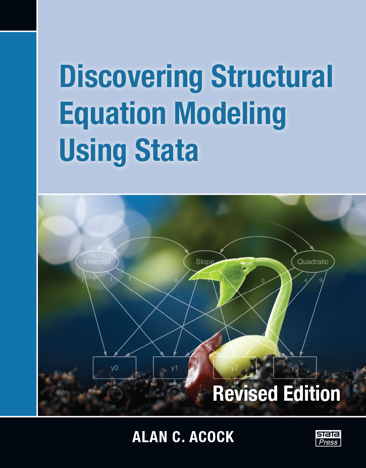
Discovering Structural Equation Modeling Using Stata, Revised Edition
106,000원
Author: Alan C. Acock Publisher: Stata Press Copyright: 2013 ISBN-13: 978-1-59718-139-6 Pages: 306; paperback
Author index
Subject index
Errata
Download the datasets used in this book
Review from the Stata Journal
Supplements: Answers to exercises
Discovering Structural Equation Modeling Using Stata, Revised Edition, by Alan Acock, successfully introduces both the statistical principles involved in structural equation modeling (SEM) and the use of Stata to fit these models. The book uses an application-based approach to teaching SEM. Acock demonstrates how to fit a wide variety of models that fall within the SEM framework and provides datasets that enable the reader to follow along with each example. As each type of model is discussed, concepts such as identification, handling of missing data, model evaluation, and interpretation are covered in detail.
In Stata, structural equation models can be fit using the command language or the graphical user interface (GUI) for SEM, known as the SEM Builder. The book demonstrates both of these approaches. Throughout the text, the examples use the sem command. Each chapter also includes brief discussions on drawing the appropriate path diagram and performing estimation from within the SEM Builder. A more in-depth coverage of the SEM Builder is given in one of the book’s appendixes.
The first two chapters introduce the building blocks of SEM. Chapter 1 begins with overviews of Cronbach’s alpha as a measure of reliability and of exploratory factor analysis. Then, building on these concepts, Acock demonstrates how to perform confirmatory factor analysis, discusses a variety of statistics available for assessing the fit of the model, and shows a more general measurement of reliability that is based on confirmatory factor analysis. Chapter 2 focuses on using SEM to perform path analysis. It includes examples of mediation, moderation, cross-lagged panel models, and nonrecursive models.
Chapter 3 demonstrates how to combine the topics covered in the first two chapters to fit full structural equation models. The use of modification indices to guide model modification and computation of direct, indirect, and total effects for full structural equation models are also covered.
Chapter 4 details the application of SEM to growth curve modeling. After introducing the basic linear latent growth curve model, Acock extends this to more complex cases such as the inclusion of quadratic terms, time-varying covariates, and time-invariant covariates.
In chapter 5, Acock discusses testing for differences across groups in SEM. He introduces the specialized sem syntax for multiple-group models and discusses the intricacies of testing for group differences for the different types of models presented in the preceding chapters.
The Revised Edition includes output, syntax, and instructions for fitting models with the SEM Builder that have been updated for Stata 13.
Discovering Structural Equation Modeling Using Stata, Revised Edition is an excellent resource both for those who are new to SEM and for those who are familiar with SEM but new to fitting these models in Stata. It is useful as a text for courses covering SEM as well as for researchers performing SEM.
Alan Acock is a sociologist and a University Distinguished Professor in the School of Social and Behavioral Health Sciences at Oregon State University. He was also recognized as the Alumni Distinguished Professor based on his work with students. He has published more than 130 articles in leading journals across the social and behavioral sciences, including Structural Equation Modeling, Psychological Bulletin, Multivariate Behavioral Research, Journal of Gerontology, Journal of Adolescence, American Journal of Public Health, American Sociological Review, Journal of Marriage and Family, Social Forces, Educational and Psychological Measurement, Journal of Politics, Prevention Science, American Journal of Preventive Medicine, and many others. He also authored the text A Gentle Introduction to Stata.
Dedication
1.2 The "do not even think about it" approach
1.3 The principal component factor analysis approach
1.4 Alpha reliability for our nine-item scale
1.5 Generating a factor score rather than a mean or summative score
1.6 What can CFA add?
1.7 Fitting a CFA model
1.8 Interpreting and presenting CFA results
1.9 Assessing goodness of fit
1.9.2 Final model and estimating scale reliability
1.10.2 Estimating a two-factor model
1.12 Extensions and what is next
1.13 Exercises
1.A Using the SEM Builder to run a CFA
1.A.2 Estimating the model
2.2 Path model terminology
2.2.2 A hypothetical path model
2.4 Estimating a model with correlated residuals
2.4.2 Strengthening our path model and adding covariates
2.6 Testing equality of coefficients
2.7 A cross-lagged panel design
2.8 Moderation
2.9 Nonrecursive models
2.9.2 Stability of a nonrecursive model
2.9.3 Model constraints
2.9.4 Equality constraints
2.B Using the SEM Builder to run path models
3.2 The classic example of a structural equation model
3.2.2 Fitting a full structural equation model
3.2.3 Modifying our model
3.2.4 Indirect effects
3.4 Programming constraints
3.5 Structural model with formative indicators
3.5.2 Multiple indicators, multiple causes model
4.2 A simple growth curve model
4.3 Identifying a growth curve model
4.3.2 Identifying a quadratic growth curve
4.4.2 Graphic representation of individual trajectories (optional)
4.4.3 Intraclass correlation (ICC) (optional)
4.4.4 Fitting a latent growth curve
4.4.5 Adding correlated adjacent error terms
4.4.6 Adding a quadratic latent slope growth factor
4.4.7 Adding a quadratic latent slope and correlating adjacent error terms
4.6.2 Interpreting a model with time-invariant and time-varying covariates
4.8 Exercises
5.2 The range of applications of Stata’s multiple-group comparisons with sem
5.2.2 A measurement model
5.2.3 A full structural equation model
5.3.2 Step 2: Testing for invariant loadings
5.3.3 Step 3: Testing for an equal loadings and equal errorvariances model
5.3.4 Testing for equal intercepts
5.3.5 Comparison of models
5.3.6 Step 4: Comparison of means
5.3.7 Step 5: Comparison of variances and covariance of latent variables
5.4.2 Fitting the model with the SEM Builder
5.4.3 A standardized solution
5.4.4 Constructing tables for publications
5.6 Exercises
A.2 Menus for Windows, Unix, and Mac
A.2.2 The vertical drawing toolbar
A.4 Drawing an SEM model
A.5 Fitting a structural equation model
A.6 Postestimation commands
A.7 Clearing preferences and restoring the defaults


